R mini-course: week 2 notes
timothy leffel may26/2017
Same format as last week: exercises and additional discussion interleaved throughout. But this time, I’d recommend starting a blank R script and typing your responses into it. That way if you want feedback, you can just send me the .R file with your solutions (where applicable), including commented lines that explain what you’re doing and why you’re doing it (example here). I’ll send you back a file that has all of your original code, plus some comments and code from me. (note: another good way to share code would be with an R-Fiddle – see the note on R-Fiddle on the course page for instructions)
Also for next week, I want everyone (who’s so compelled) to identify a dataset they’d be interested in exploring, and save it to the directory you’re storing your files for this class in. It’s definitely best if the data is in .csv format, but it doesn’t have to be. Before the regular notes, section 0 gives a quick guide on why and how to find a dataset of interest.
0. for next week: everyone obtain a dataset
Since R was designed to be used for data analysis, you’ll only understand why R works the way it does – and more importantly, what it can do for you – by practicing writing R code that manipulates rectangular datasets.
The best way to learn R is to use R. In my experience, the best way to motivate yourself to use R is to identify a topic that (i) has some kind of quantitative data associated with it; that (ii) you know how to find a dataset pertaining to; and that (iii) you have a genuine interest in understanding at a deeper level.
Since we all work in social science, there’s lots of candidates for (i) and (ii) – even if one doesn’t come to mind, ask a few colleagues and I’m sure someone will have some thoughts. But criterion (iii) can be harder to satisfy. Even so, I think it’s crucial – you’ll get bored of and/or frustrated with playing around with mtcars and iris reeeeeal quickly (trust me).
I’d actually go as far as to argue that when it comes to learning how to code in R, (iii) is more important than points (i) and (ii), because if you have a topic that satisfies (iii) but neither of the first two, then you can spend time thinking about how to code up simulations to model the phenomenon you’re interested in. At the same time I’m sure everyone has a genuine interest in getting done with their work faster (more time for twitter :p), so a good dataset might be something work-related that satisfies (iii) in virtue of you being interested in finishing your work faster and consequently having more free time.
Fortunately, the internet has many, many, many datasets to offer. For a shocking array of topics, you can google “datasets on X” and find interesting spreadsheet-like sets of numbers that can be read into R and manipulated just like mtcars or iris (in case you weren’t in class: these datasets are introduced in section 1 below).
Here’s some genres you might consider:
- spreadsheets that represent repeated measurements over time, or a set of spreadsheets that you could in theory merge together, e.g.
- a project budget/expenditures table (or a collection of them);
- stock or currency trading prices;
- game-level, player-level sports data (e.g. box scores);
- longitudinal data from an experimental(y) study; or
- your personal budget!
- a set of survey responses your team has collected as part of a project
- a word list with fields for frequency, collocation, part-of-speech, etc.
- some government data about labor, income, health, healthcare, etc. – here’s links to the ‘data’ pages of the Census Bureau and the Bureau of Labor Statistics for inspiration
Here’s some questions to keep in mind when selecting a dataset:
- does it seem manageable to get acquainted with over the next few weeks? (e.g. a full GSS dataset might be too much to digest)
- will gaining familiarity with the dataset be beneficial to you, whether personally or professionally?
- are you going to lose interest in the subject matter of the dataset quickly?
- does it have a reasonable size for quick work-checking? (let’s say: between 3 and 20 columns of interest, and between 10 and 10,000 rows)
1. Working with real data
R comes with some pre-loaded datasets, which have reserved names. The two examples we’ll look at here are mtcars and iris. They’re both kinda famous datasets in the data science world, and you should be aware of them because a lot of tutorials and walkthroughs you’ll find on the web use one of them as an example. mtcars is Motor Trend data from the ’70s about various attributes of different types of cars. iris provides several measurements of 150 individual iris flowers, each of which belongs to one of three sub-species (spoiler: the measurements can be used to predict the sub-species reasonably well). This dataset was made famous by Ronald Fisher in the ’30s and is still used regularly in examples.
Most of the built-in datasets are data frames. You can access built-in datasets by their names:
head(iris, n=5)## Sepal.Length Sepal.Width Petal.Length Petal.Width Species
## 1 5.1 3.5 1.4 0.2 setosa
## 2 4.9 3.0 1.4 0.2 setosa
## 3 4.7 3.2 1.3 0.2 setosa
## 4 4.6 3.1 1.5 0.2 setosa
## 5 5.0 3.6 1.4 0.2 setosahead(mtcars, n=5)## mpg cyl disp hp drat wt qsec vs am gear carb
## Mazda RX4 21.0 6 160 110 3.90 2.620 16.46 0 1 4 4
## Mazda RX4 Wag 21.0 6 160 110 3.90 2.875 17.02 0 1 4 4
## Datsun 710 22.8 4 108 93 3.85 2.320 18.61 1 1 4 1
## Hornet 4 Drive 21.4 6 258 110 3.08 3.215 19.44 1 0 3 1
## Hornet Sportabout 18.7 8 360 175 3.15 3.440 17.02 0 0 3 2Let’s focus on mtcars. Notice that it’s not in your environment tab. That’s because there’s a bunch of built-in datasets and it’d be annoying if they were all there all the time. We can just introduce a variable and assign the dataset to it:
tim_mtcars <- mtcarsLet’s check out what the columns are:
str(tim_mtcars)## 'data.frame': 32 obs. of 11 variables:
## $ mpg : num 21 21 22.8 21.4 18.7 18.1 14.3 24.4 22.8 19.2 ...
## $ cyl : num 6 6 4 6 8 6 8 4 4 6 ...
## $ disp: num 160 160 108 258 360 ...
## $ hp : num 110 110 93 110 175 105 245 62 95 123 ...
## $ drat: num 3.9 3.9 3.85 3.08 3.15 2.76 3.21 3.69 3.92 3.92 ...
## $ wt : num 2.62 2.88 2.32 3.21 3.44 ...
## $ qsec: num 16.5 17 18.6 19.4 17 ...
## $ vs : num 0 0 1 1 0 1 0 1 1 1 ...
## $ am : num 1 1 1 0 0 0 0 0 0 0 ...
## $ gear: num 4 4 4 3 3 3 3 4 4 4 ...
## $ carb: num 4 4 1 1 2 1 4 2 2 4 ...Not super informative. But if we google around a bit, we’ll find what each of them are:
mtcars$mpg– miles per gallonmtcars$cyl– number of cylindersmtcars$disp– displacement (in\(^3\))mtcars$hp– gross horsepowermtcars$drat– rear axle ratiomtcars$wt– weight (1000lb)mtcars$qsec– 1/4 mile timemtcars$vs– V/S (V- versus Straight block, I think)mtcars$am– automatic or manual transmissionmtcars$gear– number of gearsmtcars$carb– number of carburetors
exercise: some of these columns are coded horribly. How could we improve the legibility of the data by transforming some of the columns? (hint: inspect and contemplate the column mtcars$am)
But wait, something important is missing: what are the makes and models of the cars?! Well, turns out they’re in…
rownames(tim_mtcars)## [1] "Mazda RX4" "Mazda RX4 Wag" "Datsun 710"
## [4] "Hornet 4 Drive" "Hornet Sportabout" "Valiant"
## [7] "Duster 360" "Merc 240D" "Merc 230"
## [10] "Merc 280" "Merc 280C" "Merc 450SE"
## [13] "Merc 450SL" "Merc 450SLC" "Cadillac Fleetwood"
## [16] "Lincoln Continental" "Chrysler Imperial" "Fiat 128"
## [19] "Honda Civic" "Toyota Corolla" "Toyota Corona"
## [22] "Dodge Challenger" "AMC Javelin" "Camaro Z28"
## [25] "Pontiac Firebird" "Fiat X1-9" "Porsche 914-2"
## [28] "Lotus Europa" "Ford Pantera L" "Ferrari Dino"
## [31] "Maserati Bora" "Volvo 142E"This is annoying, and in 2017 it’s not very common to actually use rownames in R. Since rownames(tim_mtcars) is a character vector, we can just move it to a column and then delete the rownames.
tim_mtcars$make_model <- rownames(tim_mtcars)
rownames(tim_mtcars) <- NULL
quick exercise: combine assignment and $ with NULL to remove a column from a data frame.
Do we have any missing values?
# one way to check would be:
sum(is.na(tim_mtcars$mpg))
sum(is.na(tim_mtcars$cyl))
sum(is.na(tim_mtcars$disp))
# ...
## [1] 0
## [1] 0
## [1] 0# a quicker way to check:
colSums(is.na(tim_mtcars))
"" # adding an empty string to make space between the two results in the output
# aaand make sure there aren't NA's that accidentally became characters
# (note "NA" is not the same as NA)
colSums(tim_mtcars=="NA")## mpg cyl disp hp drat wt
## 0 0 0 0 0 0
## qsec vs am gear carb make_model
## 0 0 0 0 0 0
## [1] ""
## mpg cyl disp hp drat wt
## 0 0 0 0 0 0
## qsec vs am gear carb make_model
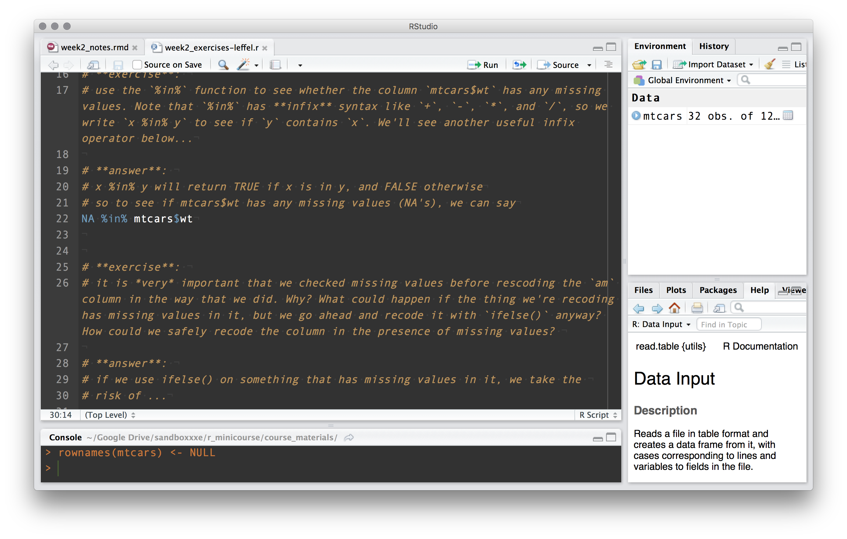
## 0 0 0 0 0 0exercise: use the %in% function to see whether the column mtcars$wt has any missing values. Note that %in% has infix syntax like +, -, *, and /, so we write x %in% y to see if y contains x (we’ll get a logical back – TRUE if x is in y, and FALSE otherwise). We’ll see another useful infix operator below…
Let’s clean up one of the columns, am, before moving on. Manual vs automatic should really not be coded as 0 or 1, since transmission is most definitely a category and not a number. We can use ifelse() to change this.
tim_mtcars$am <- ifelse(tim_mtcars$am==0, "automatic", "manual")exercise: it is very important that we checked missing values before recoding the am column in the way that we did. Why? What could happen if the thing we’re recoding has missing values in it, but we go ahead and recode it with ifelse() anyway? How could we safely recode the column in the presence of missing values?
# now let's remove tim_mtcars since we want to manipulate the original later on
rm(tim_mtcars)
2. A brief but necessary detour: packages!
Very important point: in R, packages are your friend.
One of the best things about R is that anyone can contribute helfpul, new user-defined functions and methods. These are typically bundled into a portable format called a package. Packages are just collections of functions and other stuff that aren’t part of what automatically comes with R when you install it (aka base R).
If you are using a particular package for the first time, you will have to install it, which is done with install.packages("<package name>") (note quotes around the name). Everyone should install the following packages for the class:
# install.packages("dplyr")
# install.packages("reshape2")
# install.packages("ggplot2")note: once you have a package installed, it stays installed until you update your version of R. Then, to reinstall a package, just call install.packages() on it again.
After a package is installed, you can “load” it (i.e. make its functions available for use) with library("<packagename>"). For this course, we’ll use the following packages (maybe more too).
# don't worry if you get some output here that you don't expect!
# some packages send you messages when you load them. no need for concern.
library("dplyr")
library("reshape2")
library("ggplot2")
You can see your library – a list of your installed packages – by saying library(), without an argument. You can see which packages are currently attached (“loaded”) with search(), again with no argument.
# see installed packages (will be different for everyone)
# library()

# see packages available *in current session*
search()
## [1] ".GlobalEnv" "package:ggplot2" "package:reshape2"
## [4] "package:dplyr" "package:stats" "package:graphics"
## [7] "package:grDevices" "package:utils" "package:datasets"
## [10] "package:methods" "Autoloads" "package:base"note: R Studio has lots of point-and-click tools to deal with package management and data import. Look at the R Studio IDE cheatsheet on the course page for details.
note: Check out “contributed packages” on CRAN to browse tons of cool R packages, which exist for almost any imaginable purpose!
3. The outside world (or: reading and writing external files)
3.1 read from a url
Here’s a cool word-frequency dataset:
# link to url of a word frequency dataset
link <- "http://lefft.xyz/r_minicourse/datasets/top5k-word-frequency-dot-info.csv"
# read in the dataset with defaults (header=TRUE, sep=",")
words <- read.csv(link)
# look at the first few rows
head(words, n=5)
## Rank Word PartOfSpeech Frequency Dispersion
## 1 1 the a 22038615 0.98
## 2 2 be v 12545825 0.97
## 3 3 and c 10741073 0.99
## 4 4 of i 10343885 0.97
## 5 5 a a 10144200 0.98exercise: plot frequency against rank in the words dataset. What does the pattern suggest? hint: here are links to R-Cookbook tutorials on scatterplots with ggplot2:: and scatterplots with base graphics. (fun bonus thing: after you plot frequency against rank, google “Zipf’s Law”)
3.2 read from a local file
Here’s a government education dataset I found here. I’d recommend going through the interface to download the file for practice dealing with web-based data acquisition, but no need – here’s a link you can use directly.
# i saved it to a local folder, so I can read it in like this
edu_data <- read.csv("datasets/university/postscndryunivsrvy2013dirinfo.csv")
head(edu_data[, 1:10], n=5)
names(edu_data)
## UNITID INSTNM
## 1 100654 Alabama A & M University
## 2 100663 University of Alabama at Birmingham
## 3 100690 Amridge University
## 4 100706 University of Alabama in Huntsville
## 5 100724 Alabama State University
## ADDR CITY STABBR ZIP FIPS OBEREG
## 1 4900 Meridian Street Normal AL 35762 1 5
## 2 Administration Bldg Suite 1070 Birmingham AL 35294-0110 1 5
## 3 1200 Taylor Rd Montgomery AL 36117-3553 1 5
## 4 301 Sparkman Dr Huntsville AL 35899 1 5
## 5 915 S Jackson Street Montgomery AL 36104-0271 1 5
## CHFNM CHFTITLE
## 1 Dr. Andrew Hugine, Jr. President
## 2 Ray L. Watts President
## 3 Michael Turner President
## 4 Robert A. Altenkirch President
## 5 Gwen Boyd President
## [1] "UNITID" "INSTNM" "ADDR" "CITY" "STABBR" "ZIP"
## [7] "FIPS" "OBEREG" "CHFNM" "CHFTITLE" "GENTELE" "FAXTELE"
## [13] "EIN" "OPEID" "OPEFLAG" "WEBADDR" "ADMINURL" "FAIDURL"
## [19] "APPLURL" "NPRICURL" "SECTOR" "ICLEVEL" "CONTROL" "HLOFFER"
## [25] "UGOFFER" "GROFFER" "HDEGOFR1" "DEGGRANT" "HBCU" "HOSPITAL"
## [31] "MEDICAL" "TRIBAL" "LOCALE" "OPENPUBL" "ACT" "NEWID"
## [37] "DEATHYR" "CLOSEDAT" "CYACTIVE" "POSTSEC" "PSEFLAG" "PSET4FLG"
## [43] "RPTMTH" "IALIAS" "INSTCAT" "CCBASIC" "CCIPUG" "CCIPGRAD"
## [49] "CCUGPROF" "CCENRPRF" "CCSIZSET" "CARNEGIE" "LANDGRNT" "INSTSIZE"
## [55] "CBSA" "CBSATYPE" "CSA" "NECTA" "F1SYSTYP" "F1SYSNAM"
## [61] "F1SYSCOD" "COUNTYCD" "COUNTYNM" "CNGDSTCD" "LONGITUD" "LATITUDE"3.3 reading different file types
Check out the readxl:: package, and specifically try readxl_example() to see some examples. See this vignette for some examples of reading excel files in R. (here’s a link to the data read in as crime1 and crime2)
library("readxl")
# an example of reading xls datasets
crime1 <- read_xls("datasets/crime/Crime2016EXCEL/noncampusarrest131415.xls")
crime2 <- read_xls("datasets/crime/Crime2016EXCEL/noncampuscrime131415.xls")

# see how many rows + columns each one has
dim(crime1); dim(crime2)
## [1] 11306 24## [1] 11306 46# see what columns they have in common
intersect(names(crime1), names(crime2))## [1] "UNITID_P" "INSTNM" "BRANCH" "Address" "City"
## [6] "State" "ZIP" "sector_cd" "Sector_desc" "men_total"
## [11] "women_total" "Total" "FILTER13" "FILTER14" "FILTER15"# looks like we could prooobably merge them by UNITID_P, which looks like an id
length(intersect(unique(crime1$UNITID_P), unique(crime2$UNITID_P)))## [1] 11306# could also join by INSTNM
identical(crime1$INSTNM, crime2$INSTNM)## [1] TRUE# suppose we want to join these together, matching by UNITID_P
# here's one way to do it (note that left_join() comes from dplyr::):
crime <- left_join(crime1, crime2, by=c("UNITID_P", "INSTNM"))
# now if we check it out, it's kinda a mess but it worked.
# this suggests we should've inspected the columns more thoroughly
# before joining them (bc we've probably duplicated some matching columns)exercise: look at the data wrangling cheatsheet, and determine whether left_join() was the best strategy to use here, given the crime data. How else could we have joined the datasets? What would make a left join not give us what we want?
Here’s a link to some datasets in Stata format. (and a link to the one read in as election_data)
# an example of reading a stata dta file (note we need the haven:: package)
library("haven")
election_data <- read_dta("datasets/election/bes_f2f_original_v3.0.dta")

# notice that objects read from stata maintain some of their
# idiosyncratic internal structure -- e.g. you can see the survey items
# "embedded" inside the header fields in the R Studio spreadsheet view
head(election_data, n=5)
## # A tibble: 5 x 476
## finalserialno serial wt_sel_wt wt_combined_main_capped wt_combined_main
## <dbl> <dbl> <dbl> <dbl> <dbl>
## 1 10102 2915 0.568195 0.594137 0.594137
## 2 10104 2505 1.136390 1.188274 1.188274
## 3 10107 876 1.136390 0.970153 0.970153
## 4 10109 875 1.136390 0.996799 0.996799
## 5 10202 3034 1.136390 0.968325 0.968325
## # ... with 471 more variables: wt_combined_CSES <dbl>, A1 <chr>,
## # a02 <dbl+lbl>, a03 <dbl+lbl>, m02_1 <dbl+lbl>, m02_2 <dbl+lbl>,
## # m02_3 <dbl+lbl>, m02_4 <dbl+lbl>, m02_5 <dbl+lbl>, m02_6 <dbl+lbl>,
## # m02_7 <dbl+lbl>, b01 <dbl+lbl>, b02 <dbl+lbl>, B02_other <chr>,
## # b04 <dbl+lbl>, B04_other <chr>, b05 <dbl+lbl>, b06_01 <dbl+lbl>,
## # b06_02 <dbl+lbl>, b06_03 <dbl+lbl>, b06_04 <dbl+lbl>,
## # b06_05 <dbl+lbl>, b06_06 <dbl+lbl>, b06_07 <dbl+lbl>,
## # b06_08 <dbl+lbl>, b06_09 <dbl+lbl>, b06_10 <dbl+lbl>,
## # b06_11 <dbl+lbl>, b06_12 <dbl+lbl>, b06_13 <dbl+lbl>,
## # b06_14 <dbl+lbl>, b06_15 <dbl+lbl>, b06_16 <dbl+lbl>,
## # b06_17 <dbl+lbl>, b06_18 <dbl+lbl>, b06_19 <dbl+lbl>,
## # b06_20 <dbl+lbl>, b07 <dbl+lbl>, b08_01 <dbl+lbl>, b08_02 <dbl+lbl>,
## # b08_03 <dbl+lbl>, b08_04 <dbl+lbl>, b08_05 <dbl+lbl>,
## # b08_06 <dbl+lbl>, b08_07 <dbl+lbl>, b08_08 <dbl+lbl>, b09 <dbl+lbl>,
## # b10 <dbl+lbl>, b11 <dbl+lbl>, B11_other <chr>, b12_1 <dbl+lbl>,
## # b12_2 <dbl+lbl>, b12_3 <dbl+lbl>, b12_4 <dbl+lbl>, b12_5 <dbl+lbl>,
## # b12_6 <dbl+lbl>, b13_1 <dbl+lbl>, b13_2 <dbl+lbl>, b13_3 <dbl+lbl>,
## # b13_4 <dbl+lbl>, b13_5 <dbl+lbl>, b13_6 <dbl+lbl>, b14_01 <dbl+lbl>,
## # b14_02 <dbl+lbl>, b14_03 <dbl+lbl>, b14_04 <dbl+lbl>,
## # b14_05 <dbl+lbl>, b14_06 <dbl+lbl>, b14_07 <dbl+lbl>,
## # b15_01 <dbl+lbl>, b15_02 <dbl+lbl>, b15_03 <dbl+lbl>,
## # b15_04 <dbl+lbl>, b15_05 <dbl+lbl>, b15_06 <dbl+lbl>,
## # b15_07 <dbl+lbl>, b16_01 <dbl+lbl>, b16_02 <dbl+lbl>,
## # b16_03 <dbl+lbl>, b16_04 <dbl+lbl>, b16_05 <dbl+lbl>,
## # b16_06 <dbl+lbl>, b16_07 <dbl+lbl>, b17_01 <dbl+lbl>,
## # b17_02 <dbl+lbl>, b17_03 <dbl+lbl>, b17_04 <dbl+lbl>,
## # b17_05 <dbl+lbl>, b17_06 <dbl+lbl>, b17_07 <dbl+lbl>,
## # b18_01 <dbl+lbl>, b18_02 <dbl+lbl>, b18_03 <dbl+lbl>,
## # b18_04 <dbl+lbl>, b18_05 <dbl+lbl>, b18_06 <dbl+lbl>,
## # b18_07 <dbl+lbl>, c01 <dbl+lbl>, c02_1 <dbl+lbl>, c02_2 <dbl+lbl>, ...We can even extract descriptions of each column, since they are present in the original .dta file:
# how many columns are there
numcols <- ncol(election_data)

# create an empty container to catch the column info text
election_data_colinfo <- rep(NA, times=numcols)

# for every number x between 1 and however many columns election_data has:
for (x in 1:numcols){
  # to the x'th element of
  election_data_colinfo[x] <- attributes(election_data[[x]])$label
}

# now make a df w each row as the name and description of an election_data col
election_dictionary <- data.frame(
  colname  = names(election_data),
  colinfo  = election_data_colinfo
)

# check out the first 10 -- not bad, eh?
# (reduce the zoom in R Studio to have the columns display next to each other)
head(election_dictionary, n=10)
## colname
## 1 finalserialno
## 2 serial
## 3 wt_sel_wt
## 4 wt_combined_main_capped
## 5 wt_combined_main
## 6 wt_combined_CSES
## 7 A1
## 8 a02
## 9 a03
## 10 m02_1
## colinfo
## 1 Final Serial Number
## 2 Respondent Serial Number
## 3 Selection weight (including capping)
## 4 Combined main study weight (capped selection plus capped demographic weights)
## 5 Combined main study weight (capped selection plus uncapped demographic weights)
## 6 Combined CSES weight (capped selection weight plus demographic weighting)
## 7 A1: Most important issue
## 8 Best party on most important issue
## 9 A3 How interested would you say you are in politics? Would you say you are...
## 10 Politicians don't care what people like me thinknote: here we’re using a for-loop, which is the first control structure we’ve seen. Depending on class interest, we can go deeper into looping next week. It’s an important topic, but you can do a lot of stuff in R without ever writing loops.
exercise: google “for-loops vs apply family in R”, read up about the function lapply(), and then re-write the loop above as a vectorized “loop” with sapply() or lapply().
exercise (for those interested in SPSS): find an SPSS dataset and read it in using read_spss() from the haven:: package.
3.4 simulating data
If we don’t have actual data on a topic but still want to explore it quantitatively, a good option is to randomly (but systematically!) simulate some data. Here’s an example:
# what's the probability that two of the people here have the same bday?!
# here's one strategy we could use:
# get a vector of days of the year
days <- seq(as.Date("2017-01-01"), as.Date("2017-12-31"), "days")

# define a df with 11 people, randomly assigning birthdays
birthday <- data.frame(
  # create 11 "people"
  person = paste0("person_", 1:11),
  # sample from days with replacement to assign birthdays
  bday   = sample(days, size=11, replace=TRUE)
)

# write a statement that'll be true iff two ppl have the same bday
length(unique(birthday$bday)) < nrow(birthday)
## [1] TRUEexercise: whether two people have the same birthday will vary each time you run the above, because we’re randomly sampling from days. Conceptually (i.e. without writing any code), how would we answer the question of how likely it is for two people of the 11 to share a birthday? Now, practically (i.e. by writing some code), how likely is it? Partial solution below. (hint: use a for-loop – ask me if you’re interested)
exercise: make a plot that represents the change in probability of two people having the same birthday as the size of the class increases.
# define some parameters
numsims <- 100
numppl  <- 11
# make a container to hold the simulation results
container <- rep(NA, times=numsims)
# loop over 1,2,...,numsims and generate numppl-many birthdays
for (x in 1:numsims){
  dat <- sample(days, size=numppl, replace=TRUE)
  # for each iteration, assign TRUE to the container element if we have a match
  container[x] <- length(unique(dat)) < length(dat)
}
# now get the proportion of sims where there's a common bday
sum(container==TRUE) / length(container)
# make a quick plot to see the results
ggplot2::qplot(container)
## [1] 0.15exercise: using the code block above, estimate how many people it takes to reach a 50% chance of two people having the same birthday (hint: try different values of numppl)
exercise: run the simulation a few times with numsims <- 100. Then do the same with numsims <- 10000. What’s the effect of increasing the number of simulations?
3.5 cleaning up a dataset and then writing (saving) it
Say we want to introduce info about the region of the manufacturer of each make/model in the mtcars dataset. One approach we might use: first, list all the manufacturers in the dataset, organizing them by where the maker is from (here I’m just relying on pre-existing knowledge). Then make a data frame consisting of all the unique manufacterers (mfr), and the regions associated with them.
Here’s the first step:
mfr_NA   <- c("Hornet", "Valiant", "Duster")           # unknown  manufacturer
mfr_asia <- c("Mazda", "Datsun", "Honda", "Toyota")    # asian    manufacturer
mfr_usa  <- c("Cadillac","Lincoln","Chrysler","Dodge", # american manufacturer
              "AMC","Chevrolet","Pontiac","Ford")      # european manufacturer
mfr_euro <- c("Mercedes", "Fiat", "Porsche", "Lotus",
              "Ferrari", "Maserati", "Volvo")
These vectors have all the info necessary to encode manufacturer region for the mtcars dataset. Now how should we integrate this into the dataset?! There’s more than one way we could do this, but here’s one.
Make the four mfr_* vectors into a single object…But how should we do that? A natural instinct might be to make each of them a column of a data frame…
# but if we try this we'll get an error -- **exercise**: why?
# car_regions <- data.frame(mfr_NA, mfr_asia, mfr_usa, mfr_euro)
A good way to represent this information would be as a data frame with two columns: one listing the manufacturer, and the other listing the region. Here’s how we could create such a data frame:
# make a data frame assigning regions to car types
car_regions <- data.frame(
  # the mfr_* vectors strung together
  make   = c(mfr_NA, mfr_asia, mfr_usa, mfr_euro),
  # assign regions to manufacturers, based on the mfr_* vectors and 'make'
  # the idea is to repeat the label for each value in the corresponding vector
  region = c(rep(NA,    length(mfr_NA)),   rep("asia", length(mfr_asia)),
             rep("usa", length(mfr_usa)),  rep("euro", length(mfr_euro))),
  # since we know we'll be joining this with another df, don't use factors
  stringsAsFactors=FALSE
)exercise: what’s another way we could have associated manufacturers with regions? (hint: it’s reminiscent of what we do with gear_lookup below)
exercise: how might we merge the manufacturer info in car_regions with the mtcars dataset? (hint: add a column to mtcars that has the same range of values as car_regions$make, then use a join operation from dplyr:: – see the data wrangling cheatsheet for possible join operations. Here you’ll have to create the new column by just looking at the data and saying things like, okay, a row with "Mazda RX4" should have the value "Mazda" in the new column.)
Moving on: “number of gears” (mtcars$gear) is technically a number, but practically speaking it’s kind of like a category (albeit ordered): there’s only a few possible values, and there’s no reason to think the difference between 3 and 4 gears is “comparable” to the difference between 4 and 5 gears. To avoid accidentally computing on mtcars$gear as if it were numeric, let’s recode it as character. Here is a nice, concise way to do this:
# "number of gears" is a category but currently coded as numeric

# make a "lookup table" that associates values of gear with the labels we want
gear_lookup <- c(three=3, four=4, five=5)

# now combine names(), match(), and [] to recode the values how we want them
mtcars$gear <- names(gear_lookup[match(mtcars$gear, gear_lookup)])note: since we manipulated mtcars, now it shows up in the environment pane in R Studio :)
Okay, now let’s do some other stuff to the data and then save the cleaned up version.
The following block of code illustrates the utility of combining dplyr:: data manipulation operations with the forward pipe operator %>% from magrittr::. (below that is an exercise with some starter code to re-write these operations in base-R style – both dplyr/magrittr wrangling style and base wrangling style are totally legit and you should be familiar with both)
note: I don’t expect that you guys will be able to read all of this next block just yet. With some practice, you will. And once you see exactly what’s going on, then you’ll be well on your way to writing nice, pretty, precise, concise, etc. data processing workflows.
note: See the first appendix for a quick description of how magrittr::’s forward pipe operator %>% works.
# the variable 'mtcars_clean' will hold the result of piping mtcars
# into the chain mutate() %>% select() %>% rename()
mtcars_clean <- mtcars %>%
  mutate(                                             # transform some colums:
    car       = row.names(mtcars),                        # create 'car' column
    qsec      = round(qsec),                              # round qm time
    mpg       = round(mpg),                               # round mpg
    wt        = wt * 1000,                                # get weight in lbs
    am        = ifelse(am==0, "manual", "auto"),          # code as char
    musclecar = cyl >= 6 & hp > 200 & qsec < 16           # define a muscle car
  ) %>%
  select(                                             # select cols to keep
    car, am, gear, musclecar, cyl,
    hp, qsec, gear, wt, mpg
  ) %>%
  rename(                                             # make nicer colnames
    horsepower=hp, cylinders=cyl, qm_time=qsec,
    num_gears=gear, lbs=wt, transmission=am
)exercise: rewrite the block above, but instead of using the dplyr:: functions mutate() (which re-defines a column), select() (which specifies which columns to keep), and rename() (which renames columns), use base functions. (hint: below is a partial solution)
# **this block is just a hint so it doesn't get run**
mtcars_clean <- mtcars
mtcars_clean$car <- row.names(mtcars_clean)
mtcars_clean$qsec <- round(mtcars_clean$qsec)
# <-- transform the rest of the columns here
# ...

# <-- select cols to keep here
# ...

names(mtcars_clean) <- c("...") # <-- fill in desired  names
# ...
Okay, back to saving the dataset.
Now the dataset is cleaned up to our liking and now we want to use the cleaned up vesion as our official version of record (or share it with ppl). We’ll save it in a few different formats as a demo.
note: Unless you have a very good reason to do otherwise (e.g. your boss demands .xls format), it’s always best to write data frames to disk in .csv format. .csv is the closest thing to a universal format for rectangular datasets. One exception is: if your dataset is very large (anything above ~ half a gig), it makes sense to save it in a compressed format such as .rda/.RData, so that you can load it quickly in the future.
# write as .csv (the default strategy)
# note that datasets we create get filed in output/,
# and datasets we get from elsewhere get filed in datasets/
write.csv(mtcars_clean, file="output/mtcars_clean.csv", row.names=FALSE)

# ...

# then read it back in later
mtcars_csv <- read.csv("output/mtcars_clean.csv")
rm(mtcars_csv)exercise: try writing and then reading in mtcars_clean, once with row.names=FALSE, and once without it. What’s the difference? Why might we want to specify row.names=FALSE?
# write as .rda (a compressed R data file -- can include multiple objects)
save(mtcars_clean, file="output/mtcars_clean.rda")

# ...

# then we could use load() to read it back in later
# load("mtcars_clean.rda")note: sometimes it’s useful to save a “snapshot” of whatever you’re working on, so that you can shut things down and then come back later and start where you left off. You can save your entire R workspace by using save.image(file="my/desired/location/my_desired_filename.RData"), and then bring it back up with load(). I prefer not to use load() in the middle of a session though, so we won’t use it here.
# we can save a dataset in stata format
write_dta(mtcars_clean, path="output/mtcars_stata.dta", version=14)

# ...

# and then read it back in later
mtcars_stata <- read_dta("output/mtcars_stata.dta")
Aaaand finally, for our old friend excel, we’ll look at the rio:: package (for “R, i/o”, which in turn is for “R, in/out”).
Check out the vignette for the rio:: package – you’ll see examples of how you can read and save datasets in various formats, and how you can convert between different filetypes too. Here’s an example from the vignette, which I imagine could be quite useful for many of us working at NORC. (check out the output file in excel!)
# you'll get a message w instructions for installing some suggested packages --
# i recommend following them
library("rio")

# export to sheets of an Excel workbook
export(list(mtcars = mtcars, iris = iris), "output/multi.xlsx")
4. WTF why can’t I read in this dataset right?!?!
When you’re starting out, reading in an external dataset doesnt always go like you want it to…Sometimes there’s invisible half-empty columns created by excel, and that breaks the “all columns must have the same length” rule for data frames. Other times, the dataset will use a weird or confusing quoting convention or non-standard separator, and that’ll cause problems. This can be extremely frustrating, but with practice you’ll learn that there’s really only a few possible sources of problems for reading in plain-text data (I can’t speak for other formats, unfortunately).
note: I’d consider the “standard” separators to be , (comma), \t (tab), and maybe | (pipe). Sometimes you’ll see a delimited plain-text files with extensions other than “.csv” – some examples are “.txt” (for “text”) and “.tsv” (for “tab-separated values”). These can be read in with read.table(), which is actually what’s happening under the hood anyway when you use read.csv().
This kind of stuff really has to be learned on a case-by-case basis. So here’s a list of tips for problems reading in data files:
common pitfalls + sources of errors/warnings
- comma versus tab separator (specify in
sep=argument ofread.csv()) - misalignment of headers + values (check out
fill=andskip=arguments) - empty cells (again,
fill=andskip=) - quoting + separators inside quoted vals (check out
quote=andsep=) - weird comment characters (check out
comment.char=) - directories! (you can use
"../"to go up a dir level, and"folder/"to look into a folder, all in the main argument of the read call – for example the following looks up two levels, then looks into a folder called “data/” to get the file:read.csv("../../data/boosh.csv"))
the most dangerous error!
The most dangerous error is the one that R couldn’t possibly tell you about, because it’s only an “error” in the sense that there was something wrong in the file you’re reading in. The two most common cases of this in my experience are:
LEADING/TRAILING SPACES IN VALUES AND/OR COLUMN NAMES!
"dog"vs"dog "vs" dog"vs" dog "all seem the same to humans (especially if you’re using Excel), but they are not the same to a computer.- thus it’s best practice to completely eliminate spaces from column names. This has the added benefit that if you do this, you can use the convenient dollar-sign syntax for column selection (exercise: what happens if you use
$on a column that has a space in the name? what about one with a special character?)
NON-STANDARD SYMBOLS FOR “MISSINGS” OR COMMENT CHARACTERS
- sometimes data will have missing values coded as
99or-1or something else. Since there’s inconsistency across software, this can lead to the most dangerous kind of error – the silent error. - check what the comment character is of the software that created the dataset, it could be that there’s comments in the data file, but R is trying to read them as rows. If you know this to be the case, ask yourself how you should specify
comment.char,na.strings, andskiparguments in theread.*()command you use.
useful troubleshooting strategies
- look at the data file in a plain text editor (I’d highly recommend getting Sublime Text – you can use the free version forever, it’ll just ask you if you want to buy a license every once in a while)
- read the documentation of
readxl::,haven::, andrio:: - use the R Studio point-and-click data import interface (but save the code after!)
- re-open file in excel and (re-)export, this time specifying the options you want when you save as .csv.
5. Once everything’s how we want it to be…
Let’s clean up the workspace then read in mtcars_clean again.
# read it in
dat <- read.csv("output/mtcars_clean.csv")

knitr::kable(head(dat, 5))| car | transmission | num_gears | musclecar | cylinders | horsepower | qm_time | lbs | mpg |
|---|---|---|---|---|---|---|---|---|
| Mazda RX4 | auto | four | FALSE | 6 | 110 | 16 | 2620 | 21 |
| Mazda RX4 Wag | auto | four | FALSE | 6 | 110 | 17 | 2875 | 21 |
| Datsun 710 | auto | four | FALSE | 4 | 93 | 19 | 2320 | 23 |
| Hornet 4 Drive | manual | three | FALSE | 6 | 110 | 19 | 3215 | 21 |
| Hornet Sportabout | manual | three | FALSE | 8 | 175 | 17 | 3440 | 19 |
Here is some starter code that does some useful stuff. If you understand how this code works, you’ll be able to apply it to your own unique situation.
# now manipulate it in a bunch of ways

# aggregation (group-wise mean, sd, etc.)
aggregate(mpg ~ cylinders + num_gears, data=dat, FUN="mean")
## cylinders num_gears mpg
## 1 4 five 28.00000
## 2 6 five 20.00000
## 3 8 five 15.50000
## 4 4 four 26.75000
## 5 6 four 19.75000
## 6 4 three 22.00000
## 7 6 three 19.50000
## 8 8 three 14.91667# subsetting (these all do the same thing)
filter(dat, musclecar==TRUE) # filter() is from dplyr::## car transmission num_gears musclecar cylinders horsepower
## 1 Camaro Z28 manual three TRUE 8 245
## 2 Ford Pantera L auto five TRUE 8 264
## 3 Maserati Bora auto five TRUE 8 335
## qm_time lbs mpg
## 1 15 3840 13
## 2 14 3170 16
## 3 15 3570 15dat[dat$musclecar==TRUE, ] ## car transmission num_gears musclecar cylinders horsepower
## 24 Camaro Z28 manual three TRUE 8 245
## 29 Ford Pantera L auto five TRUE 8 264
## 31 Maserati Bora auto five TRUE 8 335
## qm_time lbs mpg
## 24 15 3840 13
## 29 14 3170 16
## 31 15 3570 15subset(dat, musclecar==TRUE) # subset is a base function## car transmission num_gears musclecar cylinders horsepower
## 24 Camaro Z28 manual three TRUE 8 245
## 29 Ford Pantera L auto five TRUE 8 264
## 31 Maserati Bora auto five TRUE 8 335
## qm_time lbs mpg
## 24 15 3840 13
## 29 14 3170 16
## 31 15 3570 15# contingency tables
table(dat$transmission, dat$num_gears)##
## five four three
## auto 5 8 0
## manual 0 4 15Next Week
- we look through everyone’s datasets and discuss any issues that came up
- wide- vs long-format data, reshaping data, the concept of “tidy data”
- visualizing a dataset as a class (type-along)
- visualizing your own dataset with base graphics and
ggplot2::
Appendix: the forward pipe operator %>% from magrittr::
Most R commands consist of a function applied to one or more arguments (potentially assigning the result to a variable). In the case where there’s only one argument, it can be nice to use the forward pipe operator %>%. This is part of a family of similar operators defined in the magrittr:: package, and is made use of heavily in modern dplyr:: data processing workflows.
It’s not as scary as it looks: x %>% f() is equivalent to f(x). What’s nice about this is that you can make “pipe-chains” when you want to apply a sequence of functions to a single object (dplyr::’s functions are designed for exactly this). Forward pipe-chains have the following shape:
x %>% f() %>% g() %>% h() %>% z()
Which is equivalent to:
z(h(g(f(x)))),
except that the first one is easier to read (or will become easier to read if you start using it regularly). Assuming we want to save the result of x applied to f() through z(), we can just assign the whole chain to a variable. Here’s a little example where given the schema above, x is chars, and f() and g() are unique() and length().
chars <- sample(letters, size=20, replace=TRUE)

# we could write
numUnique <- length(unique(chars))
numUnique
## [1] 13# or equivalently:
numUnique <- chars %>% unique() %>% length()
numUnique## [1] 13After reading this, go back and look at the mtcars pipe-chain above. Make any more sense now? The more you use pipes, the more natural it will feel, and the weirder it will feel to use nested function calls like length(unique()).
Appendix: writing functions
The more you use R, the more things you’ll realize you could be doing in a waaaay more efficient manner. Learning to write your own functions is a crucial step in making your workflow and data processing pipelines more efficient and less headache-inducing.
A simple example: often we have something that’s coded as a factor or a number, and we’d rather have it coded as a character.
thing1 <- factor(rep(1:3, 5), labels=c("categoryA", "categoryB", "categoryC"))

as.character(thing1)
## [1] "categoryA" "categoryB" "categoryC" "categoryA" "categoryB"
## [6] "categoryC" "categoryA" "categoryB" "categoryC" "categoryA"
## [11] "categoryB" "categoryC" "categoryA" "categoryB" "categoryC"Imagine we had several objects like thing1 and wanted to apply as.character() to each of them (e.g. because they all have the same values, but the underlying factor values are a non-uniform mess).
thing1 <- factor(rep(1:3, 5), labels=c("catA", "catB", "catC"))
thing2 <- factor(rep(4:6, 5), labels=c("catA", "catB", "catC"))
thing3 <- factor(rep(3:5, 5), labels=c("catA", "catB", "catC"))
thing4 <- factor(rep(2:4, 5), labels=c("catA", "catB", "catC"))
thing5 <- factor(rep(3:1, 5), labels=c("catA", "catB", "catC"))
We could type out as.character() each time:
thing1 <- as.character(thing1)
thing2 <- as.character(thing2)
# ...
Or we could write a function that basically just abbreviates it. That’ll save us keystrokes.
# a quick function to save us keystrokes
ac <- function(x){
  as.character(x)
}

thing1 <- ac(thing1)
thing2 <- ac(thing2)
# ...
Another example:
# saves us even more keystrokes
lu <- function(x){
  length(unique(x))
}

lu(thing3)
lu(thing4)
lu(thing5)
## [1] 3
## [1] 3
## [1] 3exercise: rewrite the body of the lu() function as a forward pipe-chain with %>% (also, it’s good practice to put require("magrittr") or require("dplyr") at the beginning of the function body since we’ll need one of those packages to use the pipe).
So what can writing functions do for you? Here’s a function that does some useful stuff. Think of it as breaking data analysis or summary into two pieces: when you define your main function, you’re defining the data analysis routine. When you actually apply the function to your data, you’re executing the analysis.
# define analysis routine
custom_summary <- function(df, group_col, measure_col){
  require("dplyr"); require("ggplot2")

  # make a lil df with just the relevant cols
  df <- data.frame(group_col=df[[group_col]], measure_col=df[[measure_col]])

  # make a table of the mean and sd of measure_col for each value of group_col
  out_table <- df %>% group_by(group_col) %>% summarize(
    avg = mean(measure_col, na.rm=TRUE),
    sd  = sd(measure_col, na.rm=TRUE)     # ... more calculations
  ) %>% data.frame()

  # make a plot the avg of measure_col for each value of group_col
  out_plot <- ggplot(out_table, aes(x=group_col, y=avg)) +
    geom_bar(stat="identity") +
    geom_errorbar(aes(ymin=avg-sd, ymax=avg+sd, width=.25)) +
    labs(x=group_col, y=paste0("mean of ", measure_col, ", +/- sd"),
         title=paste0("average ", measure_col, " by ", group_col))

  # now combine the table (out_table) and the plot (out_plot)
  # we're using a list here because these objects are very different!
  # we can also use the $ syntax on the output, which is why we give
  # both of the slots in 'out' a name ('table' and 'plot')
  out <- list(table=out_table, plot=out_plot)

  # then return 'out' as the value of the function
  # (if you don't specify return value, the default is the final printed value)
  return(out)
}
We can apply custom_summary() to mtcars in a number of ways. Summarize mtcars$mpg for each value of mtcars$gear using custom_summary(), and assign the result to the variable mpg_by_gear.
mpg_by_gear <- custom_summary(df=mtcars, group_col="gear", measure_col="mpg")Now we can look at the components of the result that we decided to return when we defined custom_summary():
# print a table
knitr::kable(mpg_by_gear$table)| group_col | avg | sd |
|---|---|---|
| five | 21.38000 | 6.658979 |
| four | 24.53333 | 5.276764 |
| three | 16.10667 | 3.371618 |
Now the plot:
# display the plot
mpg_by_gear$plot
We can repeat the process with any data frame and any combination of variables. Play around with this for a while and some ideas might come to your mind about how we could include other useful information in the return value of custom_summary().
mpg_by_cyl <- custom_summary(df=mtcars, group_col="cyl", measure_col="mpg")

# ...exercise: use our function to summarize mpg by cyl and a couple other variables. How could we apply custom_summary() to iris to understand some aspect of that dataset?
exercise (caution – this one might not be worth the time): why does the plot have “gear” on the axis title and x-axis label, but the table ends up with “group_col”? Both were specified with group_col in the definition of custom_summary(), so why don’t they display the same? (hint: read the chapter on non-standard evaluation from Wickham’s Advanced R (the whole thing’s available for free online))